481085 (2005 SA135) vs 21028 (1989 TO)

I wonder if these two mars crossing asteroids might have generated from a common body.

The asteroid 21028 (1989 TO) is itself a recognized binary asteroid (Pravec et others). The rotation period is 3.6644 hours.

This is the result of my simulation (note, Time 0 is JD 0 --> 4713 B.C.) :

Approach

• download orbital prameters from JPL Small-Body Database
• perform simulation using Mercury6 software by John Chambers
• establish a threshold rule (distance and relative velocity) for  stating that a couple of asteroids might have a common origin
• analyze results and plot using R programming environment

Orbital parameters


481085 (2005 SA135)

Classification: Mars-crossing Asteroid          SPK-ID: 2481085

[ Ephemeris | Orbit Diagram | Orbital Elements | Physical Parameters | Discovery Circumstances ]

[ show orbit diagram ]

Orbital Elements at Epoch 2458000.5 (2017-Sep-04.0) TDB Reference: JPL 10 (heliocentric ecliptic J2000)  Element Value Uncertainty (1-sigma)   Units  e .2984405268289324 8.8599e-08 a 2.334110493987974 2.4417e-08 au q 1.637517328485263 1.9453e-07 au i 21.80096788876684 1.6384e-05 deg node 340.5993513550984 1.7134e-05 deg peri 98.81719065459441 6.9324e-05 deg M 91.04532224832778 4.774e-05 deg tp 2457671.090833414662 (2016-Oct-09.59083341) 0.00017073 JED period 1302.508432528503 3.57 2.0438e-05 5.596e-08 d yr n .2763897653247032 4.3369e-09 deg/d Q 3.030703659490684 3.1704e-08 au

Orbit Determination Parameters    # obs. used (total)      243      data-arc span      4215 days (11.54 yr)      first obs. used      2005-09-11      last obs. used      2017-03-27      planetary ephem.      DE431      SB-pert. ephem.      SB431-N16      condition code      0      fit RMS      .52233      data source      ORB      producer      Otto Matic      solution date      2017-Apr-09 05:41:20   Additional Information  Earth MOID = .79863 au   Jupiter MOID = 2.52193 au   T_jup = 3.416

21028 (1989 TO)

Classification: Mars-crossing Asteroid          SPK-ID: 2021028

[ Ephemeris | Orbit Diagram | Orbital Elements | Physical Parameters | Discovery Circumstances ]

[ show orbit diagram ]

Orbital Elements at Epoch 2458000.5 (2017-Sep-04.0) TDB Reference: JPL 17 (heliocentric ecliptic J2000)  Element Value Uncertainty (1-sigma)   Units  e .2998944450657227 5.4262e-08 a 2.332990251676451 1.1059e-08 au q 1.633339434806201 1.2906e-07 au i 21.78593156617378 8.7621e-06 deg node 340.5615644130669 1.7944e-05 deg peri 98.59272923713611 2.2979e-05 deg M 263.6251062251222 1.3504e-05 deg tp 2458348.940978486229 (2018-Aug-18.44097849) 4.9949e-05 JED period 1301.570848400155 3.56 9.2546e-06 2.534e-08 d yr n .2765888621756544 1.9666e-09 deg/d Q 3.032641068546701 1.4375e-08 au

Orbit Determination Parameters    # obs. used (total)      751      data-arc span      9775 days (26.76 yr)      first obs. used      1989-10-04      last obs. used      2016-07-09      planetary ephem.      DE431      SB-pert. ephem.      SB431-N16      condition code      0      fit RMS      .43258      data source      ORB      producer      Otto Matic      solution date      2017-Apr-05 23:49:35   Additional Information  Earth MOID = .795177 au   Jupiter MOID = 2.52435 au   T_jup = 3.417

Simulation setup

Let's try to investigate the last 1d8 days (about 274000 years), output interval every 100 days.

N-body algorithm:  Conservative Bulirsch-Stoer

This simulation will generate a file with almost 1e6 lines per asteroid.

)O+_06 Integration parameters  (WARNING: Do not delete this line!!)
) Lines beginning with `)' are ignored.
)---------------------------------------------------------------------
) Important integration parameters:
)---------------------------------------------------------------------
 algorithm (MVS, BS, BS2, RADAU, HYBRID etc) = bs2
 start time (days)= 2457800.5
 stop time (days) = -1d8
 output interval (days) = 100
 timestep (days) = 0.1
 accuracy parameter=1.d-12


Threshold rule
The following two conditions must be true at the same timestep:

• distance less that 0.0020 AU (about 1 lunar distance)
• relative velocity less than 1 meter/s

R custom program
I developed a small custom program to quickly analyze the results.

This program loads the output of the Mercury6 simulator (for every asteroid: a file with Time plus X,Y,Z and VX, VY, VZ).

For every couple of asteroids a dataframe is built: every row is associated to a specific timestep plus positions and velocities of the couple being investigated.

For every row, the distance and relative velocity is calculated and the threshold rules are checked. 

A couple of asteroids is interesting if the threshold rule is satisfied in at least one timestep. 

Once a couple is identified, a graph is built to show both distance and relative velocity.

Kind Regards,
Alessandro Odasso

2016 WF9 - a simulation based on Feb 11th orbital params

This is a simulation of asteroid 2016 WF9 based on orbital parameters published on HORIZONS Web-Interface on Feb 11th, 2017.
 
At this time, the orbital condition code is 4

Orbital Elements at Epoch 2457800.5 (2017-Feb-16.0) TDB
Reference: JPL 13 (heliocentric ecliptic J2000)

Element	Value	Uncertainty (1-sigma)	Units
e	.6580360863711519	9.9808e-06
a	2.870895540801432	8.6058e-05	au
q	.9817426747520661	8.7514e-07	au
i	14.99562014245548	9.8595e-05	deg
node	125.4263986134548	0.00019086	deg
peri	342.4337260195148	8.1316e-05	deg
M	3.004319337477674	0.00013463	deg
tp	2457785.672494105614 (2017-Feb-01.17249411)	9.1832e-05	JED
period	1776.742590373345 4.86	0.07989 0.0002187	d yr
n	.2026179830159605	9.1105e-06	deg/d
Q	4.760048406850797	0.00014269	au

This asteroid was simulated with the Mercury6 orbit simulator together with 100 virtual clones generated with the package R.

These 100 clones were generated so that their orbital parameters are normally distributed around the nominal value of asteroid 2016 WF9 and their standard deviation is almost equal to the uncertainty shown above.

Virtual Asteroids: summary

	mean	sd
a	2.8709	8.68E−05
e	0.65804	9.51E−06
i	14.9956	9.48E−05
w	342.434	8.18E−05
om	125.426	0.00019
M	3.00432	0.00014

Simulation parameters

• period simulated: past 1e8 days 
• time step 0.1 days
• ejection distance = 100 au
• N-body algorithm: Conservative Bulirsch-Stoer

Simulation results

• 1 out of 101 virtual asteroid was discarded because it would have collided with Jupiter
• 44 out of 101 virtual asteroids came from the outskirt of the solar system (i.e., there was a time in the past when their distance was more than 100 au - ejection distance from the simulator point of view), so it makes sense to think they were comets.

This is the density distribution of arrival time in the solar system:

 Actually, according to the simulation, the first cometary event was 30084 years ago and the last one occurred 273009 years ago.

Probability of being a comet

I tried to use a R survival package called survminer to display the probability of a virtual asteroid being a comet, a probability that increases as you go more and more in the past.

I built a table with three columns:

• virtual asteroid id
• year: time of arrival into solar system, or end-time of the simulation (right censored data)
• event: in case of arrival from the outskirt of the solar system, this flag is TRUE, otherwise it is FALSE coherently with column year.

The Surv function available in R can be used to convert the table in order to have a formal "survival" object and the survfit function can then be used to display a summary table showing how the various asteroids were progressively lost in favor of a comet - the lost of an asteroid is equivalent to the "death" event in a survival analysis).

These are the first lines of the survfit result:

Year(in the past)	n.risk	n.event	survival	std.err	lower 95% CI	upper 95% CI
30084	101	1	0.990	0.010	0.971	1.000
67281	100	1	0.980	0.014	0.953	1.000
70233	99	1	0.970	0.017	0.938	1.000
73898	98	1	0.960	0.019	0.923	0.999
74074	97	1	0.950	0.022	0.909	0.994
75356	96	1	0.941	0.024	0.896	0.988
80292	95	1	0.931	0.025	0.882	0.982
90790	94	1	0.921	0.027	0.870	0.975

How to read:
we started with 101 virtual asteroids, then at Year 30084 in the past we see one of them coming from the outskirt of the solar system, so we do not count it as an asteroid ...then, at Year 67281 in the past, this event occurs again ... and so on till we arrive at the last virtual asteroid being counted as a comet at Year 273009 in the past (last row not shown).

Based on this, we can draw a plot showing the probability of a virtual asteroid being a comet as a function of time:

Kind Regards,
Alessandro Odasso

Citations:

Survminer
Alboukadel Kassambara and Marcin Kosinski (2016). survminer: Drawing Survival Curves using 'ggplot2'

      Mercury Simulator - Mercury6
      J.E.Chambers (1999) "A Hybrid
      Symplectic Integrator that Permits Close Encounters between
      Massive Bodies''. Monthly Notices of the Royal Astronomical
      Society, vol 304, pp793-799.

2016 WF9 - a simulation based on Jan 5th orbital params

On Jan 5th, I downloaded the orbital parameters of asteroid 2016 WF9 and their uncertainty from the Horizons Web interface:

param     value        1-sigma

a             2.8729806 0.00200340
e             0.6582656 0.00022291
i            14.9994893 0.00329270
w        342.4286190 0.00216310
om      125.4222393 0.00428050
M        353.6898676 0.00394660

In spite of the fact that the uncertainty is still very high, I tried to make a simulation generating 100 virtual asteroids to see how many of them in the past would seem to come from a distance greater than 100 AU (cometary origin).

First, I used the R programming environment to generate the virtual asteroids.

An obvious check is that the mean value of their orbital parameters must be almost equal to the nominal values of asteroid 2016 WF9 and their standard deviation should be also almost equal to the uncertainty shown above.

In fact, looking at the virtual asteroids, I got:

a     mean     2.8729   sd 0.002
e     mean     0.6583   sd 2e-04
i      mean   14.9988   sd 0.0035
w    mean 342.4285   sd 0.0023
om  mean 125.4218   sd 0.0046
M    mean 353.6903   sd 0.004

As a second step I used the Mercury6 simulator by John E. Chambers, to simulate the past 1e8 days, output interval 100 days (hybrid algorithm).

The program simulated the behaviour of 101 asteroids (100 virtual asteroid + the "real" asteroid):

The result was that about 60 virtual asteroids would seem to have a cometary orgin (i.e. there was a time in the past when their distance from the sun was grater than 100 AU).

The earliest date is about 37500 years ago, the oldest date is constrained by the simulation period (about 275000 years ago) and the median value is 155000 years ago.

(for curiosity: the nominal orbital values of 2016 WF9 itself tells us that this can be a comet arrived 76000 years ago).

This is the graph showing the arrival time of the 60 virtual comets:

In the next weeks, when the orbit of asteroid  2016 WF9 will be better defined, I would like to repeat the simulation to see if and how much the simulation results will be different.

Kind Regards,
Alessandro Odasso


Citations

      Mercury Simulator - Mercury6
      J.E.Chambers (1999) ``A Hybrid
      Symplectic Integrator that Permits Close Encounters between
      Massive Bodies''. Monthly Notices of the Royal Astronomical
      Society, vol 304, pp793-799.

Asteroid H mag vs perihelium - ternary maps

Inspired by these beautiful examples, I have tried to use the ggtern R package to draw a few ternary maps showing how the H mag of various asteroid families varies as a function of q, i.e. the perihelium distance.

As usual, the starting point ...

Extreme TNOs - H mag

Let's apply the same approach described in the previous posts to the TNOs.

I downloaded some days ago a list of 2298 TNOs from the Horizons Web-Interface.

After reading it in an R dataframe, I have plotted the Spearman correlation versus Tisserand parameter with respect to a generic body with ap varying between 20 AU and 1000 AU. Important: I added a filter so to include ONLY asteroids with T <=3 ... this implies that the numerosity of the asteroids is not constant along this plot.

 

After some trials, it seems to me that there is a moderate correlation (better: anti-correlation) for ap = 324 AU (red vertical line).

This is visible in a rough but clear way if you just make a boxplot showing the different H mag distributions in the first and second half of the Tisserand range.

It must be said that the total number of TNOs in this plot is only 45: so I am not sure whether this is significant.

It must also be said that these 45 asteroids are very interesting: among them we can find Sedna and other famous Extreme TNOs that are being studied extensively because their orbits might have been shaped by an unknown massive planet waiting to be discovered.

We can note that the 45 asteroids have a>136 aU and e>0.677

> tapply(z$a,list(z$T324),min)
    FALSE      TRUE
 30.12661 136.09255
> tapply(z$e,list(z$T324),min)
    FALSE      TRUE
0.0000000 0.6776645

Another interesting aspect is described below.

45 TNOs - H Mag depends on Tisserand vs outer planets

Let's calculate the Tisserand parameter Tn with respect to Neptune.

After that we can flag every asteroid TNOs as Tn_le_3 or Tn_gt_3 depending on whether Tn is less than 3 or greater.

Furthermore: we repeat this process for Uranus, Saturn and Jupiter. 

In the end, every asteroid is flagged as follows:

• Neptune:  Tn_le_3 or Tn_gt_3
• Uranus - Tu_le_3 or Tu_gt_3
• Saturn -  Ts_le_3 or Ts_gt_3
• Jupiter - Tj_le_3 or Tj_gt_3

Of course, following the same convention, all our 45 TNOs have T324_le_3: this is how we chose them.

This is the boxplot showing H mag of the 45 TNOs depending on the combination of the above flags:

As you see, something quite peculiar (at least for me!) is going on:

• the brightest TNOs are those who have any Tisserand parameter with respect to outer planets greater than 3.
• when Neptune comes in (I mean: Tn<le_3), the asteroids get darker
• when Neptune and Uranus come in ... the asteroids get darker
• when Neptune, Uranus and Saturn come in ... same as above ... only 1 asteroid.
• when also Jupiter come in ... we find the darkest TNOs of this group of 45 TNOs.

This is something that I can not explain: 

• is this an expected / known result?
• is it a ... statistical fluke?

Cheers,

Alessandro Odasso

 

 

Amor - a summary plot of H vs Tisserand's parameter - Tp < 3

This post continues from the previous one.

Let's take again the plot H  mag vs Tisserand's parameter with respect to Earth (ap=1 AU). 

ONLY those Amors with TEarth<3

We have already seen this plot, we just add a few labels to count them:

We have also seen that most of these Amors have also Tisserand's parameter with respect to Jupiter, Venus and Mars <  3 (actually, I refer to it as "Mars" but the exact value for which there was a relative greater correlation between H mag and Tisserand's parameter was ap = 1.65 AU).

A possible question is:how are these asteroids distributed  in the various TEarth quartiles?

For graphical purposes, I introduce the following abbreviations:

• Tm = TRUE - Tisserand's parameter with respect to Mercury < 3
• Tv = TRUE - Tisserand's parameter with respect to Venus < 3
• Tma = TRUE - Tisserand's parameter with respect to Mars (better: ap =1.65 aU) < 3

This is the result:

I do not know enough about statistic to say that the above is really significant, but I can give you my feeling.

It seems to me that:

• in TEarth quartile Q2, Q3 and Q4: those Amors having Tma < 3 (red) tend to be brighter than the others not having Tm or Tv < 3 (green)
• in TEarth quartile Q1 and Q2: those Amors having Tma < 3 and Tv < 3 (yellow) tend to be slightly darker than those having only Tma < 3 (red)
• in TEarth quartile Q1: those 79 Amors having Tm<3 (and also Tv and Tma <3) tend to be the brightest.

Below, you can see a table showing the numerosity (as also shown in the labels displayed in the plot) and the median and sd of every group:

Numerosity

> t(tapply(pe$H,list(pe$tsquartile,pe$Tm:pe$Tv:pe$Tma),length))
                  [-0.15,2.82] (2.82,2.93] (2.93,2.97] (2.97,3]
FALSE:FALSE:FALSE           NA           4          33       79
FALSE:FALSE:TRUE           213         871         884      838
FALSE:TRUE:FALSE             1           2          NA       NA
FALSE:TRUE:TRUE            624          40          NA       NA
TRUE:FALSE:FALSE            NA          NA          NA       NA
TRUE:FALSE:TRUE             NA          NA          NA       NA
TRUE:TRUE:FALSE             NA          NA          NA       NA
TRUE:TRUE:TRUE              79          NA          NA       NA

Median

> t(tapply(pe$H,list(pe$tsquartile,pe$Tm:pe$Tv:pe$Tma),median))
                  [-0.15,2.82] (2.82,2.93] (2.93,2.97] (2.97,3]
FALSE:FALSE:FALSE           NA       23.85        24.0     24.6
FALSE:FALSE:TRUE          19.7       20.60        22.9     23.6
FALSE:TRUE:FALSE          23.6       24.15          NA       NA
FALSE:TRUE:TRUE           20.1       23.10          NA       NA
TRUE:FALSE:FALSE            NA          NA          NA       NA
TRUE:FALSE:TRUE             NA          NA          NA       NA
TRUE:TRUE:FALSE             NA          NA          NA       NA
TRUE:TRUE:TRUE            19.2          NA          NA       NA

Standard deviation

> t(tapply(pe$H,list(pe$tsquartile,pe$Tm:pe$Tv:pe$Tma),sd))
                  [-0.15,2.82] (2.82,2.93] (2.93,2.97] (2.97,3]
FALSE:FALSE:FALSE           NA   0.9832238    1.984962 2.098781
FALSE:FALSE:TRUE      2.153851   2.4985271    2.592066 2.609018
FALSE:TRUE:FALSE            NA   1.2020815          NA       NA
FALSE:TRUE:TRUE       2.234240   2.1410988          NA       NA
TRUE:FALSE:FALSE            NA          NA          NA       NA
TRUE:FALSE:TRUE             NA          NA          NA       NA
TRUE:TRUE:FALSE             NA          NA          NA       NA
TRUE:TRUE:TRUE        1.967811          NA          NA       NA

Cheers,

Alessandro Odasso

Amor - H mag vs Tisserand (ONLY Tp < 3)

I refer to my previous post. Following some comments from Alan Harris, I have re-drawn the relation H mag vs Tisserand with respect to a planet with generic semi-major axis ap taking into account ONLY those asteroids that have Tp < 3.

Amor - Method 1
Method based on Spearman correlation.

Having filtered only those asteroids that have Tp < 3, I have to restrict the range where the semimajor axis ap can vary:

0.35 AU <= ap <= 3 AU

For the purpose of the next plot, this is a table showing the orbital parameters of the planets:

	Semimajor Axis (AU)	Orbital Period (yr)	Orbital Speed (km/s)	Orbital Eccentricity (e)	Inclination of Orbit to Ecliptic (°)	Rotation Period (days)	Inclination of Equator to Orbit (°)
Mercury	0.3871	0.2408	47.9	0.206	7.00	58.65	0
Venus	0.7233	0.6152	35.0	0.007	3.39	-243.01*	177.3
Earth	1.000	1	29.8	0.017	0.00	0.997	23.4
Mars	1.5273	1.8809	24.1	0.093	1.85	1.026	25.2
Jupiter	5.2028	11.862	13.1	0.048	1.31	0.410	3.1
Saturn	9.5388	29.458	9.6	0.056	2.49	0.426	26.7
Uranus	19.1914	84.01	6.8	0.046	0.77	-0.746*	97.9
Neptune	30.0611	164.79	5.4	0.010	1.77	0.718	29.6

 This is the plot showing the correlation between H mag and Tp calculated for various values of semimajor axis ap expressed in AU:

I have added the following vertical lines, showing the ap of the planets:

• blue line - Mercury
• green line - Venus
• red line - Earth
• magenta line - Mars

I wonder whether the planets are truly responsible for the peaks that we see in this plot.

This is probably true for Earth, because the peak is located at ap = 1.0 AU

Not clear if we can claim that this is true for Mercury and Venus.

In the case of Mars, this is less convincing: the peak next to Mars is not located at ap=1.52 AU but slightly greater.

Boxplot for ap=0.3871 AU

we only have 79 asteroids, with tp < 3, belonging to these Tp quartiles.
> summary(p1$tsquartile)
[-0.299,2.34]   (2.34,2.58]   (2.58,2.89]      (2.89,3]
           20            20            19            20

Boxplot for ap=0.7233  AU
In this case we have 746 asteroids with T<3
> summary(p1$tsquartile)
[-0.198,2.68]   (2.68,2.85]   (2.85,2.94]      (2.94,3]
          187           186           187           186

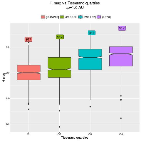
Boxplot for ap=1.0 AU
In this case we have 3668 asteroids with T<3
> summary(p1$tsquartile)
[-0.15,2.82]  (2.82,2.93]  (2.93,2.97]     (2.97,3]
         917          917          917          917

Boxplot for ap=1.65 AU
It turns out that the peak next to Mars semimajor axis is located at about ap= 1.65 AU
In this case we have 5617 asteroids with T<3
> summary(p1$tsquartile)
[-0.0765,2.66]    (2.66,2.75]    (2.75,2.83]       (2.83,3]
          1405           1404           1404           1404

Finally, I would like to see if the method2 based on Chi-squared test gives a similar answer.

Amor - Method2
Method based on Chi-squared statistic (see previous post):

In this case the effect of Mercury (if real) can not be seen.
Much more clear, if real, the effect of Earth and Mars ... some doubts about Venus.


Cheers,
Alessandro Odasso